Imagine yourself as a realtor trying to use math to make your job easier. A new community has been built, but only the square footage and price of each home has been released. Now, you are looking to use this information to predict the prices of other new houses purely based on the square footage. To do this, you need to devise a model, or a function which takes square footage as an input, and calculates the house cost as an output. But this can’t be any random function, it must also accurately predict the prices of the houses down the street.

For this task, you could choose from a wide variety of function “types” ranging from linear functions all the way to complex trigonometric functions. But for simplicity, you decide on using a linear model. Now the goal is to find the line that best fits your data points.

We first have to create a metric that quantifies how wrong or how far away our line is from the best possible line, known as an error or loss function. There are many different options for this, but a popular and easy choice is Mean Squared Error (MSE):

$$MSE = \frac{1}{n} \sum_{i=1}^{n} (y_i - \hat{y}_i)^2$$

Where:

• $n$ is the number of data points
• $y_i$ is the actual value (price of the house)
• $\hat{y}_i$ is the predicted value (price of the house based on the model)

MSE works by going over each data point and subtracting the predicted value from the actual value and then squaring the result.

Now the goal is to minimize the $MSE$ by finding the optimal slope and intercept of the line. By minimizing the error function, we can find the line that best fits our data points.

Minimizing the error function

In order to minimize the error function and find the optimal line, we need to write the error function in terms of the slope and intercept.

First we denote the slope as $m$ and the intercept as $b$. The predicted value can then be written as:

$$\hat{y}_i = m{x_i} + b$$

Where $x_i$ is the square footage of the house.

Then we can substitute this expression for $\hat{y}_i$ into the MSE formula:

$$MSE = \frac{1}{n} \sum_{i=1}^{n} (y_i - (m{x_i} + b))^2$$

Solving the error function

Since linear regression is a relatively simple task (only involving one input and one output with a simple linear model), it is possible to directly solve for the optimal slope and intercept using calculus.

The idea is that since MSE is a quadratic function, its minima can be found by setting the derivative with respect to $m$ and $b$ to zero and solving the resulting equations.

This is guaranteed to give us the minimum point / vertex of the MSE function because a quadratic function is convex (shaped like a U) and therefore has only one minima and no saddle points.

If we take a look at a normal quadratic function:

We can see that it has a single minima at $x = 0$. At this point, the derivative of the function is zero, and this makes sense because the slope of the tangent line at this point is horizontal.

Real world example

Let's say our house data points are as follows:

Now we want to model the best line that fits these data points.

We know the predicted value can be written as:

$$\hat{y}_i = mx_i + b$$

Therefore, we can evaluate the MSE function for our data points:

$$E(m, b) = \frac{1}{4}(((300000 - (1500m + b))^2  + ...   (600000 - (3000m + b))^2)$$

To find the optimal values of $m$ and $b$, we take the partial derivatives of $E(m, b)$ with respect to $m$ and $b$, set them to zero, and solve the resulting equations.

$$\frac{\partial E}{\partial m} = -\frac{1}{2} \sum_{i=1}^{n} x_i (y_i - (mx_i + b)) = 0$$

Applying this to our data points:

$$\frac{\partial E}{\partial m} = -\frac{1}{2}(1500(300000 - (1500m + b)) + ... + 3000(600000 - (3000m + b))) = 0$$

Now we can take the partial derivative with respect to $b$:

$$\frac{\partial E}{\partial b} = -\frac{1}{2} \sum_{i=1}^{n} (y_i - (mx_i + b)) = 0$$

And applying this to our data points:

$$\frac{\partial E}{\partial b} = -\frac{1}{2}((300000 - (1500m + b)) + ... + (600000 - (3000m + b))) = 0$$

Now we have a system of two equations with two unknowns ($m$ and $b$) that we can solve simultaneously. Solving these equations gives us the optimal values for $m$ and $b$:

$$\frac{\partial E}{\partial m} = -\frac{1}{2}(4300000000 - 21500000m - 9000b) = 0$$

$$\frac{\partial E}{\partial b} = -\frac{1}{2}(1800000 - 9000m - 4b) = 0$$

Simplifying these equations, we get:

$$10750000m + 4500b = 2150000000$$

$$4500m + 2b = 900000$$

Solving this system of equations, we find:

$$m = 200$$

$$b = 0$$

Verifying the results, we can see that this line perfectly fits our data points:

Generalizing to multiple features

In real world scenarios, there are often multiple features that can influence the output. For example, in addition to square footage, factors such as the number of bedrooms, location, and age of the house can also impact its price.

Now instead of a single value as our input, we have a vector of features and instead of a single slope $m$ we have a vector of weights $w$.

The predicted value can now be written as:

$$\hat{y}_i = w_1x_{i1} + w_2x_{i2} + ... + w_kx_{ik} + b$$

Or in vector form:

$$\hat{y}_i = w \cdot x_i + b$$

Where:

• $w$ is the vector of weights
• $x_i$ is the vector of features for the $i^{th}$ data point
• $b$ is the intercept

Multiple outputs

So far we have only considered the case of a single output (house price). However, in many scenarios, there may be multiple outputs to predict. For example, in addition to predicting the price of a house, we may also want to predict its rental value, or we might want to return a vector of probabilities for different classes in a classification problem.

In such cases, the model can be extended to handle mutiple outputs by using a weight matrix $W$ instead of a weight vector $w$. The y-intercept is then extended to be a bias vector $b$.

The predicted value can now be written as:

$$\hat{y}_i = W x_i + b$$

Where:

• $W$ is the weight matrix
• $x_i$ is the vector of features for the $i^{th}$ data point
• $b$ is the bias vector

Does this look familiar? This is exactly how a single layer of a neural network operates! Each neuron in the layer computes a weighted sum of the inputs, adds a bias, and produces an output. By stacking multiple layers of such neurons, we can create deep neural networks capable of learning complex patterns in data.

Neural Networks

A neural network is essentially a series of layers, where each layer consists of multiple neurons. Each neuron takes in multiple inputs, applies weights to them, adds a bias, and then passes the result through an activation function to produce an output.

If we go back to the multiple features section, we can see that this is exactly the equation for a single neuron in a neural network layer.

$$\hat{y}_i = w \cdot x_i + b$$

A single neuron gets its value from the dot product of the weights and the inputs, plus a bias.

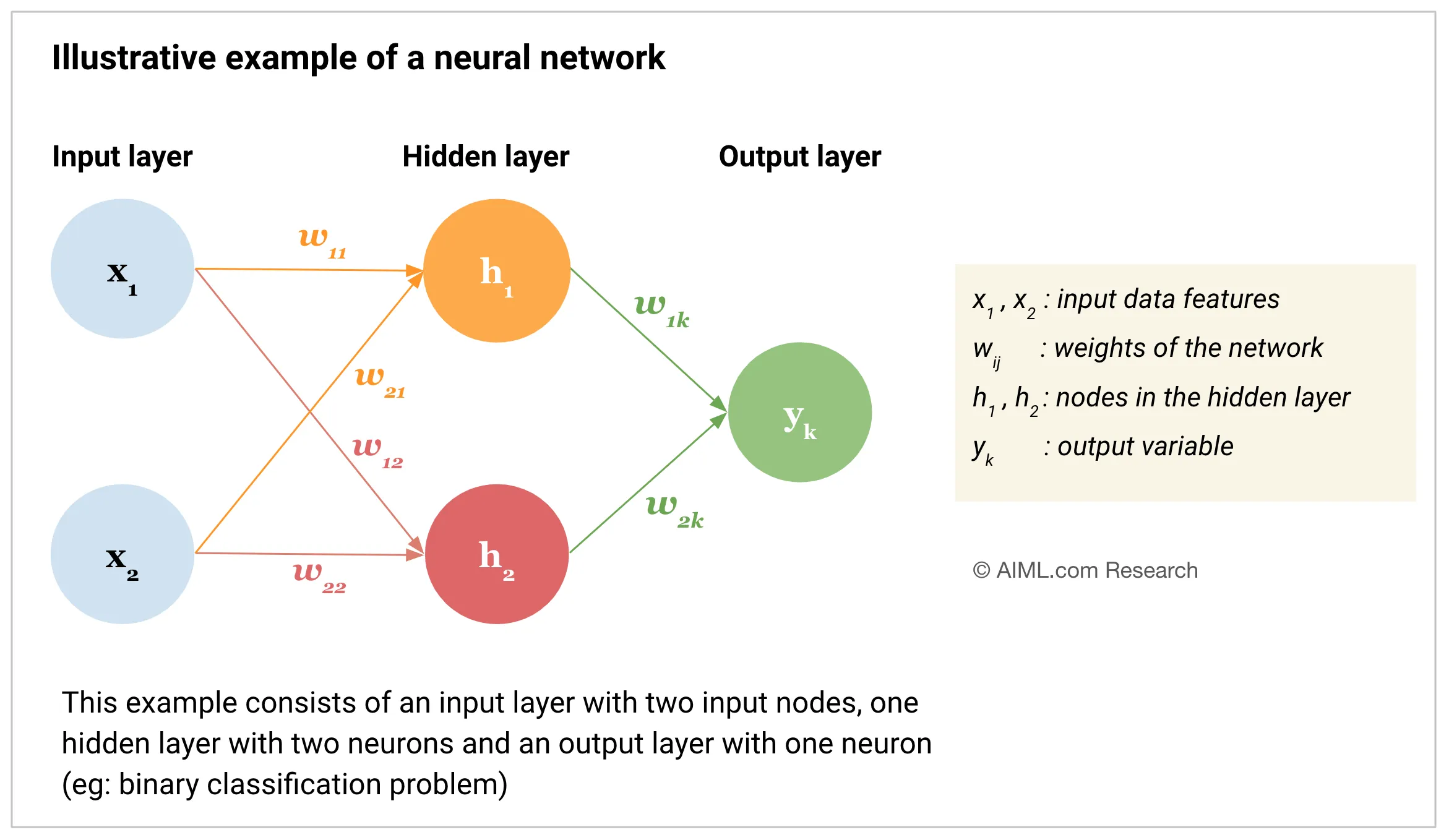
After repeating this for multiple neurons in a layer, we get a vector of outputs. In effect, each layer of a neural network is performing a linear transformation on the input data.

Activation Functions

However, if we only stack layers of linear transformations, the entire network would still be equivalent to a single linear transformation. This is where activation functions come into play. Activation functions introduce non-linearity into the model, allowing it to learn complex patterns in the data.

Some common activation functions include:

• ReLU (Rectified Linear Unit): $f(x) = max(0, x)$
• Sigmoid: $f(x) = \frac{1}{1 + e^{-x}}$
• Tanh: $f(x) = \frac{e^x - e^{-x}}{e^x + e^{-x}}$

For example, the sigmoid function maps any input value to a value between 0 and 1, which is useful for binary classification tasks:

Another cool thing about activation functions is that they can apply operations that depend on the entire input vector, not just element-wise operations. For example, the softmax function is often used in the output layer of classification networks to convert raw scores into probabilities.

$$\text{softmax}(z_i) = \frac{e^{z_i}}{\sum_{j} e^{z_j}}$$

After neurons apply their weights and biases, the activation function is applied to all elements of the output vector.

The forward pass

In a simple linear function, we can get the output by just plugging in the input values into the equation. However, in a neural network, we have multiple layers of neurons, each applying weights, biases, and activation functions. The process of passing the input data through all these layers to get the final output is known as the forward pass.

First, the input vector is passed to the first layer of neurons. Each neuron computes its output by taking the dot product of the input vector and its weight vector, adding the bias, and then applying the activation function.

This produces an output vector for the first layer, which then becomes the input vector for the next layer. This process is repeated for each layer in the network until we reach the final output layer.

In practice, the forward pass is implemented with matrix multiplications for efficiency. Multiplying the input matrix by the weight matrix of a layer yields the same result as computing the dot product for each neuron individually.

The output vector from the final layer is the prediction of the neural network and can be interpreted based on the specific task (e.g., regression, classification).

Training the neural network

Just like with our linear regression example, the goal is to find the optimal parameters that minimize the error function. In the case of linear regression, we could directly solve for the optimal slope and intercept using calculus. However, neural networks are much more complex and have many more parameters (weights and biases) to optimize, so directly solving for the optimal parameters is basically impossible.

Instead, we use an iterative optimization algorithm called gradient descent. The idea is to start with random initial values for the weights and biases, compute the error using a loss function (like MSE or cross-entropy), and then adjust the parameters in the direction that reduces the error.

We define a learning rate ($\alpha$) which determines how big of a step we take going "downhill" on the error surface. Specifically we compute the gradient of the loss function with respect to each parameter, and then change move the parameters in the opposite direction of the gradient.

Gradients and Jacobians

A simple one input one output function has a simple one value derivative, which tells us how the output changes with respect to the input. However, for a function with multiple inputs, a single value couldn't describe how the output changes with respect to each input. Instead, we use a vector of partial derivatives, known as the gradient.

The gradient of a function $f(x_1, x_2, ..., x_n)$ is a vector that contains the partial derivatives of the function with respect to each input variable:

$$\nabla f = \left[ \frac{\partial f}{\partial x_1}, \frac{\partial f}{\partial x_2}, ..., \frac{\partial f}{\partial x_n} \right]$$

If we go back to the linear regression example, we can see that the MSE function has two parameters: the slope $m$ and the intercept $b$. Therefore, the gradient of the MSE function is a vector with two components:

$$\nabla MSE = \left[ \frac{\partial MSE}{\partial m}, \frac{\partial MSE}{\partial b} \right]$$

And we solved for the optimal line by setting the gradient to zero and solving the resulting equations.

In a neural network, however, we have many more parameters, and multiple outputs as well. Now a vector can't describe how every output changes with respect to every input. Instead, we use a matrix of partial derivatives, known as the Jacobian.

The Jacobian of a vector-valued function $f: \mathbb{R}^n \rightarrow \mathbb{R}^m$ is an $m \times n$ matrix that contains the partial derivatives of each output with respect to each input:

$$J = \begin{bmatrix}
\frac{\partial f_1}{\partial x_1} & \frac{\partial f_1}{\partial x_2} & ... & \frac{\partial f_1}{\partial x_n} \\
\frac{\partial f_2}{\partial x_1} & \frac{\partial f_2}{\partial x_2} & ... & \frac{\partial f_2}{\partial x_n} \\
... & ... & ... & ... \\
\frac{\partial f_m}{\partial x_1} & \frac{\partial f_m}{\partial x_2} & ... & \frac{\partial f_m}{\partial x_n}
\end{bmatrix}$$

For the weight matrix of a neural network layer, the Jacobian is just the weight matrix itself. This makes sense because the matrix is doing a linear transformation of the input vector.

Since the loss function outputs a scalar value, it's derivative is described by a gradient vector. However for each layer in the network, includng activation functions, we need to compute the Jacobian matrix in order to understand how the output of that layer changes with respect to its inputs.

Backpropagation + Gradient Descent

Think of the loss function as a surface that maps the parameters of a neural network to a single error value. Therefore, to optimize the parameters, we need to find the lowest point on this surface.

Then, think of the gradient of the loss function as a vector that is tangent to this surface at a given point, and points in the direction of the steepest ascent. To minimize the loss, we need to move in the opposite direction of the gradient.

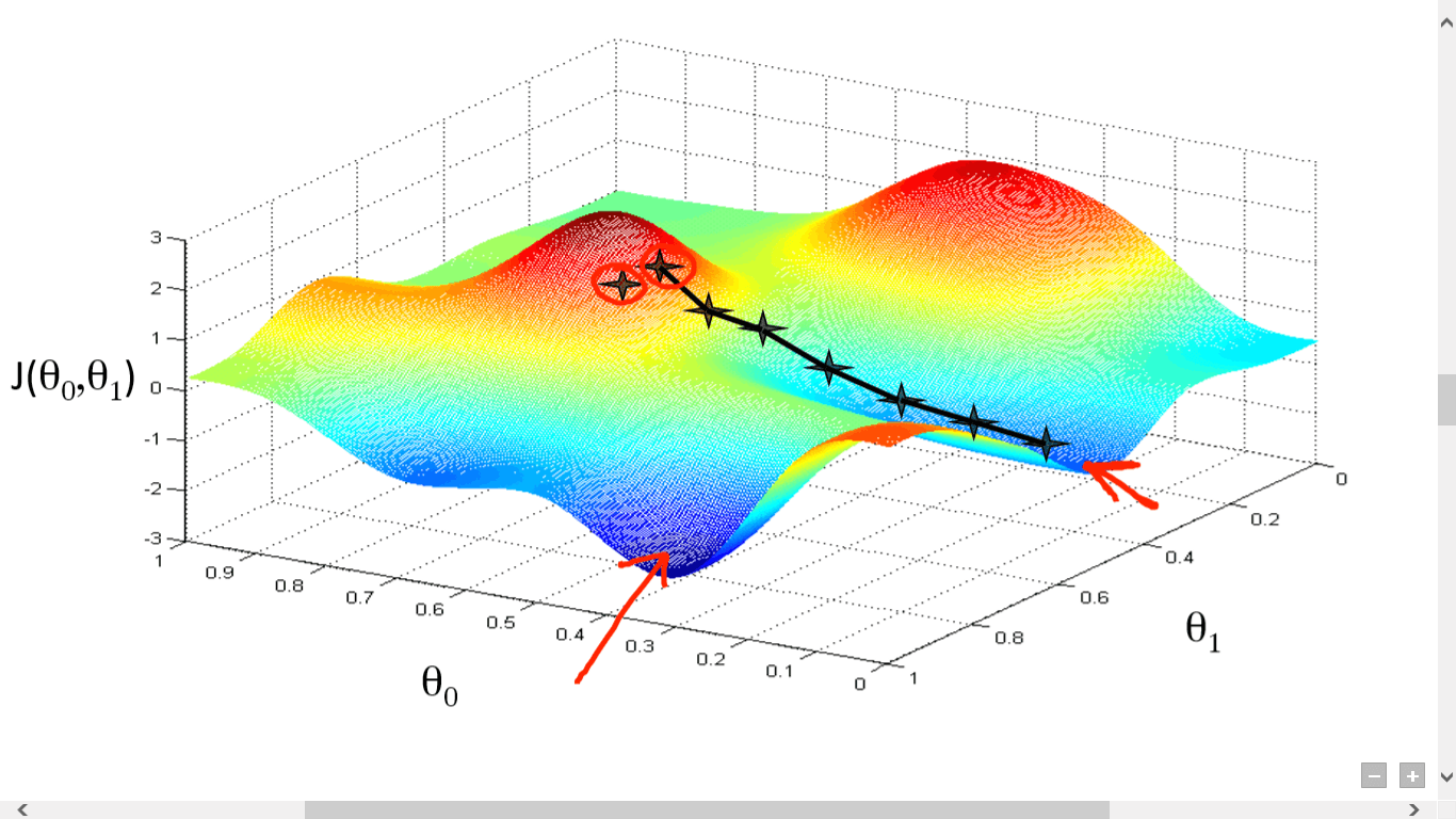
Now that we have the gradient, how do we use it to update the parameters? In practice, we don't plug in the entire model parameters into the loss function to compute the gradient. In models with millions or billions of parameters, this would be computationally infeasible. Instead, our error function only takes in the output of the model as the input, and we use the chain rule to compute the gradient of the loss function with respect to each parameter in the model.

Why does this work? Doesn't the loss function have to map our parameters to an error?

Remember that doing a forward pass involves passing the input data through each layer, each applying a linear transformation followed by a non-linear activation function. Therefore, our neural network is just a composition of functions.

Let's take a look at a simplified case of a neural network with two layers:

$$\hat{y} = f_2(W_2 f_1(W_1 x + b_1) + b_2)$$

Where:

• $x$ is the input vector
• $W_1$ and $W_2$ are the weight matrices for the first and second layers
• $b_1$ and $b_2$ are the bias vectors
• $f_1$ and $f_2$ are the activation functions for the first and second layers
• $\hat{y}$ is the output vector

Now let's say we have a loss function $L(\hat{y}, y)$ that takes in the predicted output $\hat{y}$ and the true output $y$ and outputs a scalar error value.

The gradient of the loss function with respect to the outputs is then:

$$\nabla_{\hat{y}} L = \frac{\partial L}{ \partial \hat{y}}$$

But $y_i$ is a function of $W_2$, $b_2$, $W_1$, and $b_1$. Therefore, we can use the chain rule to compute the gradient of the loss function with respect to each parameter.

For the second layer activation function ($f_2$):

$$\nabla_{z_2} L = \nabla_{\hat{y}} L \cdot J_{f_2}(z_2)$$

Remember that the activation function maps a vector to a vector, so its derivative is described by a Jacobian matrix. Since a matrix multiplied by a vector results in another vector, the result is still a vector, which in this case is the gradient of the loss function with respect to the input of the activation function.

$$\nabla_{z_2} L = \frac{\partial L}{ \partial \hat{y}} \cdot \frac{ \partial \hat{y}}{\partial z_2}$$

$$\nabla_{z_2} L = \frac{\partial L}{ \partial z_2}$$

Working backwards, we can now compute the gradient of the loss function with respect to the weights and biases of the second layer.

Currently, we have the gradient of the loss with respect to the input of the second activation.

$$\nabla_{z_2} L = \frac{\partial L}{ \partial z_2}$$

Our goal is to find the gradient with respect to the weights, and then the biases, for the second layer. We want:

$$\nabla_{W_2} L = \frac{\partial L}{ \partial W_2}$$

Now if we want to use the chain rule, we need to calculate $\frac{\partial z_2}{\partial W_2}$, because by the chain rule we have:

$$\nabla_{W_2} L = \frac{\partial L}{ \partial z_2} \cdot \frac{\partial z_2}{\partial W_2}$$

So how do we calculate $\frac{\partial z_2}{\partial W_2}$? First, let's write the equation for the layer. Recall the equation from the forward pass:

$$z_2 = W_2 a_1 + b_2$$

How does each element of the vector $z_2$ change with respect to each element of the matrix $W_2$?

The $i^{th}$ element of $z_2$ is computed as:

$$z_{2i} = W_{2i} \cdot a_1 + b_{2i}$$

Where $W_{2i}$ is the $i^{th}$ row of the weight matrix $W_2$.

So, the gradient of $z_{2i}$ with respect to the weights in the $i^{th}$ row of $W_2$ is just the input vector $a_1$. Therefore, the jacobian of $z_{2i}$ with respect to $W_2$ is just 0 in all rows except for the $i^{th}$ row, which is equal to $a_1$.

If we repeat this for each element of $z_2$ we get a rank-3 tensor representing the derivative of $z_2$ with respect to $W_2$. However, only the $i^{th}$ row of the $i^{th}$ matrix/slice is non-zero, and is equal to the input vector $a_1$.

Now what happens when we multiply this tensor by the gradient vector $\nabla_{z_2} L$?

Multiplying by a tensor can yield different results depending on how the multiplication is defined. In this case, we want to define the multiplication such that we get a matrix of the same shape as $W_2$. Let 's say the shape of $W_2$ is $(m, n)$, meaning it has $m$ rows and $n$ columns. Then the shape of $a_1$ is $(n, 1)$, and the shape of $z_2$ is $(m, 1)$.

This makes sense because the weight matrix transformed our input column vector of n neurons from the previous layer into an output column vector of m neurons for the next layer.

This means that the shape of $\nabla_{z_2} L$ is also $(m, 1)$, since it has the same shape as $z_2$, because this describes how the loss changes with respect to each output neuron.

When multiplying the vector $\nabla_{z_2} L$ with the tensor $\frac{\partial z_2}{\partial W_2}$, we take all rows in the same spot in the tensor and apply a special weighted sum with the gradient vector to get an output vector. Then we repeat this for each row in the tensor to get a matrix.

What does it mean to take all rows in the same spot in the tensor? This just means taking the $i^{th}$ row from each slice/matrix of the tensor. Now to apply our special weighted sum, we take the first element of the gradient vector and multiply it by the row we are on in the first slice, then take the second element of the gradient vector and multiply it by the same row in the second slice, and so on. Finally we sum all these resulting vectors together to get a single output vector.

Now we repeat this operation for all the remaining rows to capture how the loss changes with respect to each row of $W_2$. The result is a matrix of the same shape as $W_2$, which is exactly what we wanted.

The trick

Recall that:

Visualizing this, the Jacobian of $z_2i$ with respect to $W_2$ looks like:

$$\frac{\partial z_{2i}}{\partial W_2} = \begin{bmatrix}
0 & 0 & ... & 0 \\
0 & 0 & ... & 0 \\
... & ... & ... & ... \\
a_{1_1} & a_{1_2} & ... & a_{1_3} \\
... & ... & ... & ... \\
0 & 0 & ... & 0 \\
\end{bmatrix}$$

Where the $i^{th}$ row is equal to the input vector $a_1$.

This is just one slice of the tensor $\frac{\partial z_2}{\partial W_2}$, and we have that the $i^{th}$ row of the $i^{th}$ slice is equal to $a_1$, while all other rows are zero.

So, when we do our weighted sum multiplication over the rows of the tensor, we can see that the only non-zero contribution to the sum for the $i^{th}$ row comes from the $i^{th}$ slice, because all other slices have a zero row in that position.

Therefore, the result of the weighted sum for the $i^{th}$ row is just the $i^{th}$ element of the gradient vector $\nabla_{z_2} L$ multiplied by the input vector $a_1$.

Visualizing the output matrix, we have:

$$\nabla_{W_2} L = \begin{bmatrix}
\nabla_{z_2 L_1} \cdot a_1 \\
\nabla_{z_2 L_2} \cdot a_1 \\
... \\
\nabla_{z_2 L_m} \cdot a_1 \\
\end{bmatrix}$$

Where $\nabla_{z_2 L_i}$ is the $i^{th}$ element of the gradient vector $\nabla_{z_2} L$.

If we were to expand each row out, we would get:

$$\nabla_{W_2} L = \begin{bmatrix}
\nabla_{z_2 L_1} \cdot a_{1_1} & \nabla_{z_2 L_1} \cdot a_{1_2} & ... & \nabla_{z_2 L_1} \cdot a_{1_n} \\
\nabla_{z_2 L_2} \cdot a_{1_1} & \nabla_{z_2 L_2} \cdot a_{1_2} & ... & \nabla_{z_2 L_2} \cdot a_{1_n} \\
... & ... & ... & ... \\
\nabla_{z_2 L_m} \cdot a_{1_1} & \nabla_{z_2 L_m} \cdot a_{1_2} & ... & \nabla_{z_2 L_m} \cdot a_{1_n} \\
\end{bmatrix}$$

Does this look familiar? This is just the outer product of the gradient vector $\nabla_{z_2} L$ and the input vector $a_1$!

The outer product

Normally when we multiply a vector of shape (m, 1) with a vector of shape (n, 1), we get a single scalar value representing the dot product of the two. However, if we want to get a matrix of shape (m, n), we can use the outer product.

This involves multiplying each element of the first vector with each element of the second vector to get a matrix where the element at position (i, j) is equal to the product of the i-th element of the first vector and the j-th element of the second vector. To do this we can just transpose the second vector to have shape (1, n) and then do a normal matrix multiplication.

The goal is basically to have one row vector and one column vector, so when we multiply them together, we get a matrix.

Therefore, we can compute the gradient of the loss function with respect to the weights of the second layer as:

$$\nabla_{W_2} L = \nabla_{z_2} L \otimes a_1$$

Where $\otimes$ denotes the outer product. This can be rewritten using the transpose as:

$$\nabla_{W_2} L = \nabla_{z_2} L \cdot a_1^T$$

The bias

Recall the equation for the second layer:

$$z_2 = W_2 a_1 + b_2$$

Now the goal is to compute the gradient of the loss function with respect to the bias vector $b_2$.

We want:

$$\nabla_{b_2} L = \frac{\partial L}{ \partial b_2}$$

And we have the gradient of the loss function with respect to the pre-activation output of the second layer:

$$\nabla_{z_2} L = \frac{\partial L}{ \partial z_2}$$

Now, to get the gradient with respect to the bias, we need to compute $\frac{\partial z_2}{\partial b_2}$, because by the chain rule we have:

$$\nabla_{b_2} L = \frac{\partial L}{ \partial z_2} \cdot \frac{\partial z_2}{\partial b_2}$$

Calculating $\frac{\partial z_2}{\partial b_2}$ is straightforward. If we treat $W_2 a_1$ as constants, then the derivative of $z_2$ with respect to $b_2$ is just 1 for each element, because each element of $z_2$ changes by the same amount as the corresponding element of $b_2$.

Therefore, the Jacobian of $z_2$ with respect to $b_2$ is just the identity matrix:

$$\frac{\partial z_2}{\partial b_2} = I$$

Where $I$ is the identity matrix of shape (m, m).

Now when we multiply the gradient vector $\nabla_{z_2} L$ by the identity matrix, we just get the same vector back:

$$\nabla_{b_2} L = \nabla_{z_2} L \cdot I = \nabla_{z_2} L$$

So the gradient of the loss function with respect to the bias vector $b_2$ is just equal to the gradient of the loss function with respect to the pre-activation output of the second layer:

$$\nabla_{b_2} L = \nabla_{z_2} L$$

Continuing backwards

Now that we have the gradients with respect to the weights and biases of the second layer, we can continue this process backwards through the network to compute the gradients for all layers. First, we need to compute the gradient of the loss function with respect to the input ($a1$) of the second layer.

Formally, we need to find $\nabla_{a_1} L = \frac{\partial L}{ \partial a_1}$. Since we already have $\nabla_{z_2} L = \frac{\partial L}{ \partial z_2}$, by the chain rule we need to compute $\frac{\partial z_2}{\partial a_1}$.

Again, we can use the equation for the second layer:

$$z_2 = W_2 a_1 + b_2$$

The Jacobian of $z_2$ with respect to $a_1$ is just the weight matrix $W_2$, because each element of $z_2$ changes by the same amount as the corresponding element of $a_1$ scaled by the weights.

We know that the shape of $W_2$ is (m, n), and the shape of $\nabla_{z_2} L$ is (m, 1). Therefore, we can't multiply them directly because the inner dimensions don't match (m != 1). However, if we transpose $W_2$ to have shape (n, m), then the inner dimensions match (1 == 1) and we can do the multiplication to get a vector of shape (n, 1).

Then, the gradient of the loss function with respect to the input of the second layer is:

$$\nabla_{a_1} L = \nabla_{z_2} L \cdot W_2^T$$

Then we can compute the gradient with respect to the weights and biases of the first layer using the same method as before.

$$\nabla_{W_1} L = \nabla_{a_1} L \cdot x^T$$

$$\nabla_{b_1} L = \nabla_{a_1} L$$

Where $x$ is the input vector to the network.

Now that we have the gradients for all layers, we can update the weights and biases using gradient descent.

$$W_2 = W_2 - \alpha \nabla_{W_2} L$$

$$b_2 = b_2 - \alpha \nabla_{b_2} L$$

Both the weights and biases are updated by subtracting the learning rate multiplied by the respective gradients.

Backpropagation Algorithm

From what we have done so far, we can make some psuedocode for the backpropagation algorithm:

layers = [ (W1, b1, f1), (W2, b2, f2), ..., (Wn, bn, fn) ]  # List of layers with weights, biases, and activation functions

# forward pass
layers_output = []  # To store outputs of each layer
input = x          # Initial input to the network

for (W, b, f) in layers:
    z = W * input + b  # Linear transformation
    a = f(z)           # Activation function
    layers_output.append((z, a))  # Store pre-activation and post-activation outputs
    input = a         # Output becomes input for next layer

a2 = input  # Final output after last layer

# Compute loss
L = loss(a2, y)  # Loss function comparing output to true labels
# Backward pass
# Compute gradients for output layer

loss_grad = loss_derivative(a2, y)  # Gradient of loss with respect to output

for index in range(len(layers)-1, -1, -1):
    W, b, f = layers[index]
    z = layers_output[index][0]  # Pre-activation output of current layer
    f_jacobian = activation_jacobian(f, z)  # Jacobian of activation function

    # Gradient with respect to pre-activation output
    grad_z = loss_grad * f_jacobian

    # Gradients with respect to weights and biases
    grad_W = grad_z * input.T  # Outer product
    grad_b = grad_z             # Gradient with respect to bias

    # Update weights and biases
    W -= learning_rate * grad_W
    b -= learning_rate * grad_b

    # Update loss gradient for next layer
    loss_grad = grad_z * W.T  # Backpropagate through weights

Iterating over the dataset

There are multiple strategies for updating the weights and biases using gradient descent + backprop. The approach we covered is known as stochastic gradient descent (SGD), where we update the parameters after computing the gradients for a single data point. Then we loop over all the data points in the dataset, updating the parameters after each one.

In practice, we often use mini-batches of data points instead of a single point to compute the gradients. This is known as mini-batch gradient descent, where we update the parameters using the average of the gradients for a small batch of data points. This is a good balance between the efficiency of using the entire dataset (batch gradient descent) and the noise reduction of using a single data point (SGD).

After going through all data points (or mini-batches), we have completed one epoch of training. We can then repeat this process for multiple epochs until the model converges to a good set of parameters and low enough error.

Overfitting and Regularization

A major challenge in training neural networks is overfitting, where the model learns to memorize the training data instead of generalizing to new data. This can happen when the model is too complex relative to the amount of training data, or when the training process goes on for too long.

To combat overfitting, we can use various regularization techniques:

• L2 Regularization: This involves adding a penalty term to the loss function that is proportional to the sum of the squares of the weights. This encourages the model to learn smaller weights, which can help prevent overfitting.

$$L_{reg} = L + \lambda \sum_{i} W_i^2$$

• Dropout: This involves randomly "dropping out" (setting to zero) a fraction of the neurons in the network during training. This forces the model to learn redundant representations and prevents it from relying too heavily on any single neuron.
• Early Stopping: This involves monitoring the performance of the model on a validation set during training, and stopping the training process when the performance starts to degrade. This prevents the model from overfitting to the training data.

Summary

In this post, we started with a simple linear regression example and derived the optimal parameters using calculus. We then generalized this to multiple features and outputs, which led us to the concept of neural networks. We saw how each layer of a neural network performs a linear transformation followed by a non-linear activation function.