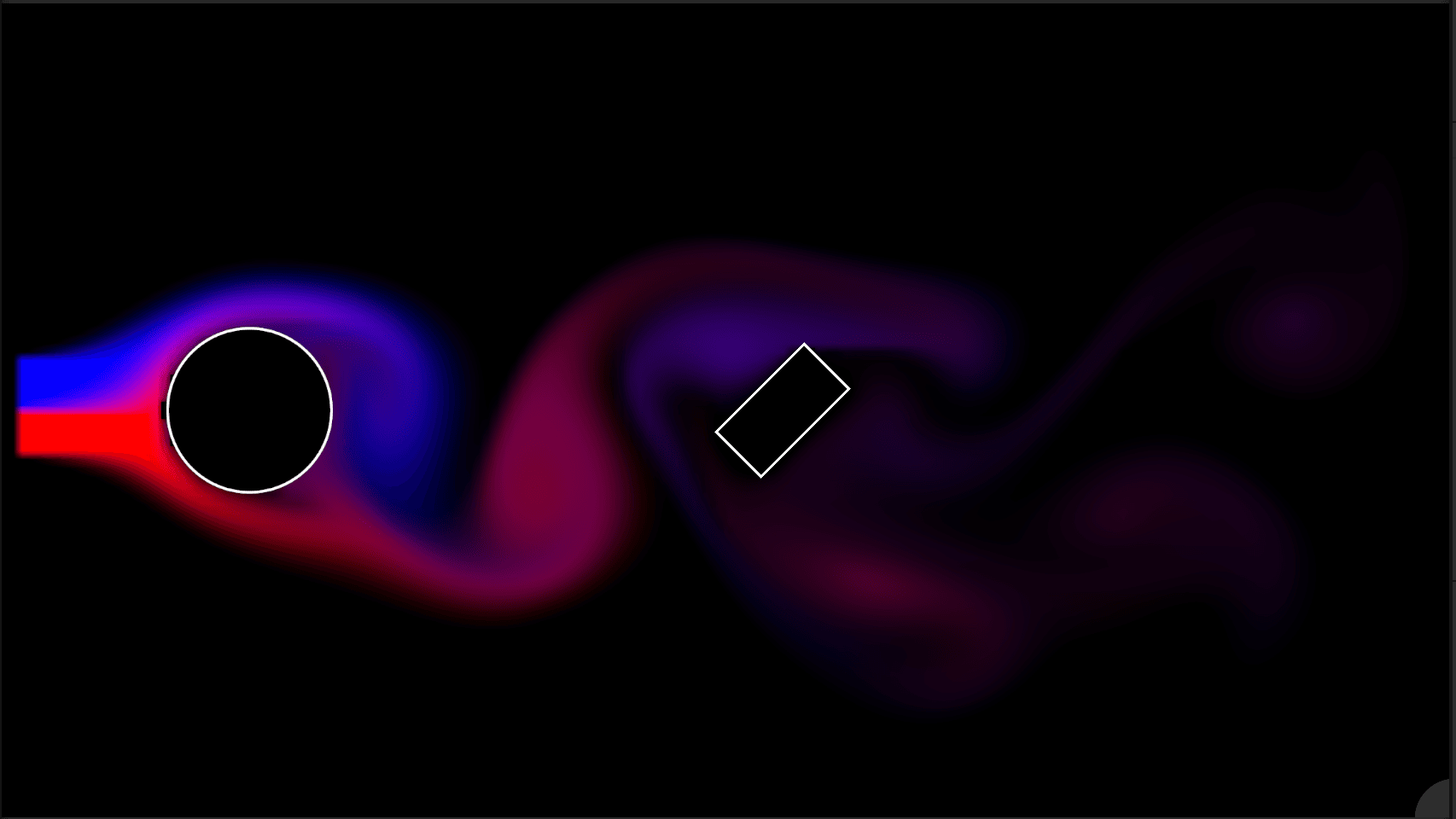
How are computers even able to simulate and render fluids? With so many molecules and extremely complex looking patterns, how is it possible for a computer with digital logic to even attempt this task?

A fluid itself is made up of an enormous number of molecules interacting with one another in the microscopic scale. Tracking the behavior of each and every molecule is basically impossible due to the sheer number of them, but we can still describe the behavior of a fluid as a whole using mathematical equations.

The first step is to let go of the idea of there being discrete molecules, and instead think of the fluid as a continuous substance that fills up space. By thinking of the fluid as a continuum, we can use vector and scalar fields to describe the properties of the fluid at every point in space.

As with most physical systems, these fields are governed by differential equations that describe how they change over time and space. The fundamental equations that govern fluid dynamics are known as the Navier-Stokes equations.

The Navier-Stokes Equations

We start with the most fundamental law of Newtonian mechanics:

$$\mathbf{F} = m \mathbf{a}$$

Since we are dealing with fluids, we need to express this equation in terms of fluid properties. We can start by expressing mass ($m$) as the product of density ($\rho$) and volume ($V$), and acceleration ($\mathbf{a}$) as the material derivative of velocity ($\frac{D \mathbf{u}}{D t}$):

$$\mathbf{F} = \rho V \frac{D \mathbf{u}}{D t}$$

The Material Derivative

What is the material derivative? Consider a tiny packet moving through the fluid's velocity field. As the packet moves, it experiences acceleration due to forces applied on it over time. However, if it enters a new region of the fluid which is moving at a different velocity, it will also experience acceleration due to this change in velocity as it moves through space. The key is understanding that for the packets to experience the correct forces we need to account for the acceleration due to both time and space changes in velocity. Moreover, we will soon see how these packets represent quantities that form the fluid and are affected by its velocity such as dye, smoke density, or temperature.

The material derivative is written as follows:

$$\frac{D \mathbf{u}}{D t} = \frac{\partial \mathbf{u}}{\partial t} + (\mathbf{u} \cdot \nabla) \mathbf{u}$$

The first term ($\frac{\partial \mathbf{u}}{\partial t}$) represents the local change in velocity over time at a fixed point. The second term ($(\mathbf{u} \cdot \nabla) \mathbf{u}$) represents the convective change in velocity as the fluid packet moves through space. Specifically, the ($\nabla$) operator returns the gradient of the velocity field (a matrix describing the velocity vector changes in each direction). Then, we multiply this gradient matrix by the velocity vector at our point ($\mathbf{u}$) to get a new vector that describes how the velocity changes in the direction of the fluid's motion. Finally, applying this operation on ($\mathbf{u}$) gives us the convective acceleration.

Forces Acting on the Fluid

Now that we have described the acceleration of a fluid packet, we can express the forces acting on it. In fluid dynamics, the main forces we consider are pressure forces, viscous forces, and external forces (like gravity).

Physically, as fluid molecules move around, they collide with one another. Taking into account the average effect of these collisions, it's clear that particles will spread out from regions with a lot of particles to regions with fewer particles due to the sheer fact that more particles = more collisions. To describe this in our continuum model, we introduce the concept of pressure. Pressure is a scalar field that represents the force exerted

To actually calculate this force, we need the gradient of the pressure field ($\nabla p$) which describes how the pressure changes in space. Pressure is a force applied over an area, so taking the gradient of pressure, we get units of pressure per distance or force over volume. Then, to get force, we multiply the pressure gradient by the volume. Since we want the fluid to accelerate from regions of high pressure to low pressure, we take the negative of the pressure gradient. This yields the pressure force as $-V\nabla p$, where $V$ is the area.

Viscous forces arise due to the internal friction between fluid layers as they move past one another. This frictional force tends to resist motion and smooth out velocity differences within the fluid. The viscous force can be modeled using the Laplacian of the velocity field ($\nabla^2 \mathbf{u}$). The laplacian operator sums the second spatial derivatives of the velocity fields, giving us a vector that describes how our velocity differs from the neighboring velocities. This captures the idea that viscosity acts to reduce velocity differences between adjacent fluid layers. Kinematic viscosity ($\nu$) quantifies the fluid's resistance to flow. With units of $\frac{m^2}{s}$, multiplying it by the laplacian (which has units of velocity per meter squared $\frac{1}{s \cdot m}$) gives us acceleration due to viscous forces. To get force from acceleration, we multiply by mass ($\rho V$), yielding the viscous force as $\rho V \nu \nabla^2 \mathbf{u}$.

Finally, we have external forces such as gravity that act on the fluid. We write these forces as $\rho V \mathbf{f}$, where $\mathbf{f}$ is the external force per unit mass (acceleration).

Combining all these forces and applying Newton's second law, we get:

$$\rho V \frac{D \mathbf{u}}{D t} = -V \nabla p + \rho V \nu \nabla^2 \mathbf{u} + \rho V \mathbf{f}$$

Then dividing through by the mass ($\rho V$) and expanding the material derivative, we arrive at the Navier-Stokes equation for incompressible fluids:

$$\frac{\partial \mathbf{u}}{\partial t} + (\mathbf{u} \cdot \nabla) \mathbf{u} = -\frac{1}{\rho} \nabla p + \nu \nabla^2 \mathbf{u} + \mathbf{f}$$

The Incompressibility Condition

In addition to this, we also have the incompressibility condition for incompressible fluids:

$$\nabla \cdot \mathbf{u} = 0$$

This equation states that the divergence of the velocity field is zero, meaning that the fluid's volume does not change as it flows. Intuitively, it means that we can't have any points where fluid is either being created or destroyed; the amount of fluid entering a region must equal the amount leaving it.

Simulation Approaches

These equations are notoriously complex and difficult to solve, especially for turbulent flows. Although they describe how fluids behave, they don't really help us actually simulate and solve fluid dynamics problems practically.

As a result, many different algorithms and even entire fields of study have emerged to tackle the challenge of simulating fluids. Most of the current approaches lie in 3 main categories:

1. Eulerian-Methods: These methods divide the simulation space into a discrete grid or mesh, and track fluid properties (velocity, density, pressure) at each grid point. The fluid flows through the grid, and the equations are solved at each grid cell. Examples include Finite Difference Methods (FDM), Finite Volume Methods (FVM), and Finite Element Methods (FEM).
2. Lagrangian-Methods: These methods track individual fluid particles as they move through space. Each particle carries its own properties, and the equations are solved for each particle. Examples include Smoothed Particle Hydrodynamics (SPH).
3. Hybrid-Methods: These methods combine elements of both Eulerian and Lagrangian approaches. For example, the Fluid-Implicit Particle (FLIP) method uses particles to represent the fluid, but also employs a grid to solve the incompressibility constraint. This allows for more accurate simulations of complex fluid behavior.

Coding the Simulation

Most fluid simulations used in both research and computer graphics today are based on the Eulerian approach due to its stability and efficiency. In this approach, we discretize the simulation space into a grid, and track fluid properties at each grid cell. I also chose Unity to

The setup

For each fluid property (velocity, density, pressure, etc.) we create a 2D array to represent the grid. For all the scalar values, we can interpret each value as being located at the center of each grid cell. However, for velocities, we use a staggered grid approach known as a MAC (Marker-And-Cell) grid. In this approach, we store the horizontal velocity components ($u$) at the left and right faces of each grid cell, and the vertical velocity components ($v$) at the top and bottom faces of each grid cell. This arrangement helps to prevent numerical instabilities and ensures that the incompressibility condition is satisfied more accurately.

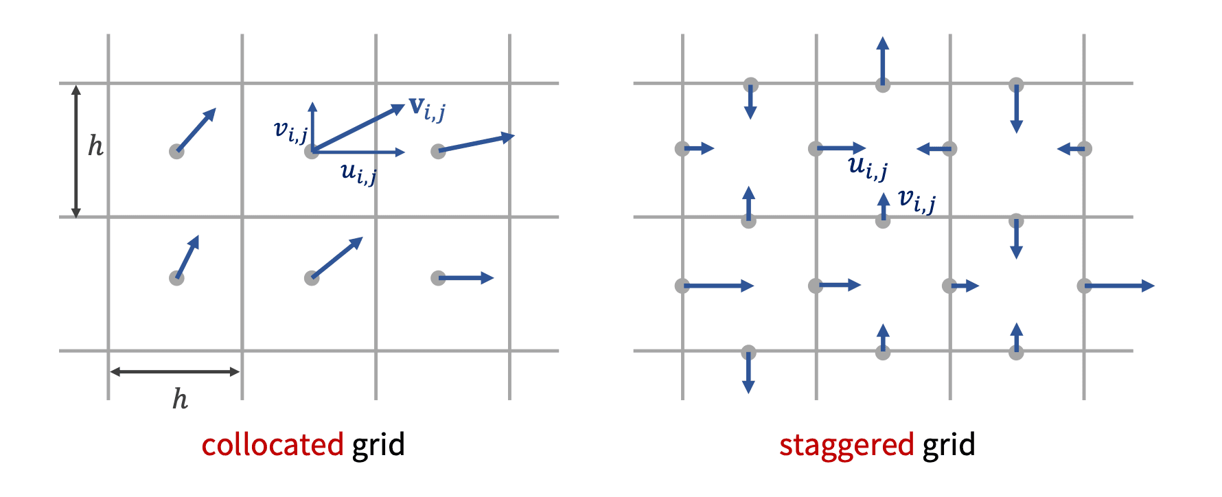
Here, the horizontal velocities are labeled ( $u$ ) and the vertical velocities are labeled ( $v$ ), and since both are stored between cells, there will be one extra row/column for each velocity component. So we store the horizontal velocities in a ( $(N+1) \times N$ ) array, and the vertical velocities in a ( $N \times (N+1)$ ) array, where ( $N$ ) is the number of cells along one dimension.

Solving for incompressibility

To enforce the incompressibility condition, we need to ensure that the divergence of the velocity field is zero at each grid cell. The divergence at a grid cell can be approximated using finite differences:

$$\nabla \cdot \mathbf{u} \approx \frac{u_{i+1,j} - u_{i,j}}{\Delta x} + \frac{v_{i,j+1} - v_{i,j}}{\Delta y}$$

Where ( $\Delta x$ ) and ( $\Delta y$ ) are the grid cell sizes in the x and y directions, respectively. (In this case, I'm using square cells with size cellSize.)

This approximation just calculates the net flow into the cell in both directions, and the goal is to make this value zero for every cell.

This may seem pretty straightforward; just adjust the velocities of a cell so that the divergence is 0. However, changing the velocities around one cell affects the divergence of the cell's neighbors as well. This means that we need to solve a large system of equations to find the correct velocity adjustments for all cells simultaneously.

Lagrange Multipliers

For any velocity field, there are infinitely many ways to adjust the velocities to make the divergence zero. So how do we choose the "best" way to adjust them? In a fluid, pressure

To achieve this, we can use pressure to correct the velocities. The idea is that pressure gradients cause fluid to accelerate from high-pressure regions to low-pressure regions, which can be used to adjust the velocities to enforce incompressibility. For each cell, we iteratively calculate a pressure value ( $p_{i,j}$ ) and then update all the surrounding velocities based on the pressure gradient.

The idea is that for each cell, we look up the pressure values of its neighboring cells, then calculate the new pressure of the curent cell as :

$$p_{i,j} = \frac{1}{4} ( p_{i+1,j} + p_{i-1,j} + p_{i,j+1} + p_{i,j-1} - \rho \frac{\Delta x^2}{\Delta t} (\nabla \cdot \mathbf{u})_{i,j} )$$

This equation states that the pressure at cell ( $i,j$ ) is the average of the pressures of its four neighboring cells, minus a term that accounts for the current divergence at that cell. The term ( $\rho \frac{\Delta x^2}{\Delta t} (\nabla \cdot \mathbf{u})_{i,j}$ ) represents how much we need to adjust the pressure to reduce the divergence.

However, there is a key detail we are missing: if we want obstacles, like walls or solid objects, we need to enforce boundary conditions on the velocities and